The finite element method describes the solution of the physical problem with a discrete number of variables, typically the displacements of the nodes composing a vector u (the velocity and acceleration are respectively denoted and ). The dynamic equation of motion may be written as , where M is the mass matrix and F is the vector of difference between the external and internal (produced by the resistance of the elements) forces for the degrees of freedom. The mass matrix is typically diagonal (condensed) for explicit integration, and constant in time. But the residual force F generally depends on the displacements. The semi-discrete equation can be discretised with time increments Δt substituting with the approximation from the central-difference equation for velocity at increment i, resulting

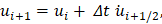
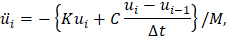
If the solution (displacements at increments and velocities at half increments) has already been computed up to step time i, then the new velocity can be explicitly computed as

As already introduced, the mass matrix is conveniently condensed to be easily inverted decoupling the algebraic equations.

Then, the central difference equation for the displacement can be used to compute the displacements at i + 1 explicitly,

The process loops again providing the evolution of the solution.

Consistency implies that the error (with respect to the exact solution) in a measure of the displacements during a single step increment has an upper bound proportional to (Δt)^k, where k ≥ 2 is the order of the local truncation error; it is 2 for the described method, implying a first order of accuracy (global error).

On the other hand, consistency does not imply the convergence of the method, where stability of the integration is also required. Explicit finite-element dynamic simulations require that the time increment be small enough to ensure a stable numerical integration. We say that the solution is conditionally stable.

This is illustrated in a simple example. Consider the free vibrations of a mass M attached to one end of a spring of elastic constant K with the other end fixed. The exact solution can be expressed as an amplitude modulated by a simple harmonic function at a natural frequency of .

The explicit central difference integration rule is of the form

where , and are the displacements (with respect to the released spring), velocities and accelerations of the mass at time increment .

Equation (2) can be used to express the velocity terms in (1) as a function of the displacements. Besides, the acceleration can also be expressed as a function of the displacements using Newton’s second law of dynamics, 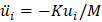, resulting

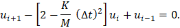
The equation describes a linear homogeneous recurrence. A solution is of the form such that α verifies the characteristic equation

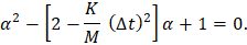
There are generally two values of α verifying the quadratic equation, and , such that the general solution of the recurrence is . The solutions of the quadratic equation are not required to be real numbers, and neither are the constants A₁ and A₂, which can be determined for specified real values of u_-1 and u₀.

In order to have a stable solution, the modulus of α in (4) must be lower than or equal to one. After a few computations the inequality is rewritten as

The natural frequency (in rad per unit time) of the simple harmonic oscillator is (previously written) and, consequently, the inequality can be expressed as

For the two first consecutive displacements of 1 and -1 the succession of values in (3) for would be 1, -1. 1, -1… If the time increment is higher, then the solution would oscillate with ever increasing amplitudes, unphysically increasing the energy of the system.

This is illustrated further for this specific problem in the figure 1, where the motion is integrated from an initial spring extension and a velocity of zero using different time increments represented with the Courant number Δt / Δt_crit. The evolution of the error is shown in figure 2. It can be observed that for a Courant number of 1.05 > 1 the error grows exponentially, while for smaller time increments it does not occur.

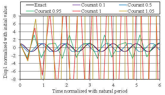
Figure 1: Explicit integration of a mass-spring system

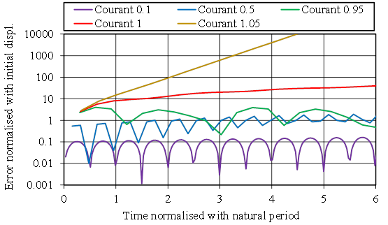
Figure 2: Error in the explicit integration of a mass-spring system

It is convenient to clarify that the error involved by the time-increment size in most models is not a matter of concern once stability is achieved. This is so because, typically, the relevant natural frequencies of the structures are orders of magnitude lower than the maximum eigenfrequency of the discretised system.

Now, assume there is a viscous damper of constant C. Since in the physical system the damping reduces the amplitude of the oscillations in time, one might be tempted to think that it can increase the critical time increment, but we will show that it is not the case, rather the opposite.

The acceleration in (1) can now be written as

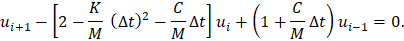
where the velocity is determined by finite differences based on the solutions at increments i and i‑1. The solution at i+1 can be explicitly determined rearranging the terms of the new recurrence

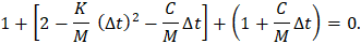
In the limit of stability, the succession 1, -1, 1, -1… would still be a solution. Despite the damping, the energy is not reduced. It is satisfied when

The time increment that solves the equation establishes the criterion for stability

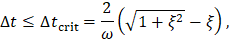
where is the fraction of critical damping. In the case of Rayleigh damping, the equivalent fraction of critical damping decreases with the eigenfrequency for the mass-proportional damping coefficient and increases with the eigenfrequency for the stiffness-proportional coefficient. Since the higher eigenfrequencies are more critical, the time increment is usually much more affected by the latter coefficient.

Similar considerations can be done for multiple degrees of freedom. In this case, the mass matrix is considered diagonal, so that it can easily be inverted (previously discussed) and the solution at a new time increment can be explicitly determined from the values at the previous increments. The spectral analysis produces the same condition (5), introducing the maximum eigenfrequency w_max of the discretised system. But solving the eigenfrequency problem is costly and impractical, and consequently the programs carry out estimations for w_max.

To illustrate this, let us consider a one-dimensional problem consisting on a rod (truss element) of length L, area A and Young's modulus E, with one end fixed. The discretised problem is similar to the problem of a mass of magnitude ρAL/2 attached to a spring of constant EA/L. The stability condition for the undamped system is

The term is the wave propagation speed c and, consequently, the stable time increment is proportional to L/c. It is worth noting that the two natural frequencies of the one-dimensional bar element without any end fixed would be zero and of the natural frequency of the bar element with one end fixed.

More generally, the maximum element eigenfrequency is an upper bound of the eigenfrequencies of the discretised system. One possibility for determining a stable time increment in an arbitrary problem is to make it proportional to L_min/c,

where L_min is the minimum characteristic element size and c is the already introduced material property. The factor depends on the element type. It is worth noting that the minimum element size conditions the time increment, thus leading to meshes that are more uniform than used in implicit methods. A physical interpretation is that the time increment should be less than the physical time required to transmit information between material points located at the nodes of the mesh. The characteristic element length depends on the element geometry and formulation.

Using smaller time increments increases the number of steps required to cover the interval of interest, increasing the number of operations and consequently the computational time.

Consider, for example, a steel structure meshed with elements of size 5 mm. The wave speed of the material is around 5000 m/s and the time increment of the simulation would be of the order of 1 µs. If the timespan of interest is 0.1 s, the number of increments required to complete the simulation would be 100,000. This is within the order of magnitude of typical explicit simulations.

Explicit integration is not only convenient for highly dynamic problems as impact, crash and shock processes. It may also be a good choice, for example, for highly nonlinear quasi-static problems where convergence is difficult and may require artificial techniques; e.g. for problems with multiple contacts that change the stiffness matrix discontinuously. It would be more practical to solve the problem by explicit integration, except that the timespan of interest may be much longer than the time increment.

In the previous example, suppose that a load is applied in 100 s. Then the required number of increments would be 100 million. If in the new scenario the response is quasi-static, then one could artificially increase the loading rate to reduce the computational cost. This a valid strategy provided that the problem remains quasi-static (energy checks are useful, verifying that the kinetic energy is negligible in comparison other energies of interest). But two other things should be considered. One is that, even if the inertia forces are negligible, time may affect the material behaviour (e.g. viscoelasticity, dependence of the plastic behaviour on strain rate, etc.). The other is that perhaps only a few elements are critical, and it might be better to act only on some elements, instead of acting globally in the model by increasing the loading rate.

It is unlikely that the elements can be removed from the mesh without affecting the results; the trick would be to increase artificially the density of the material of those particular elements to reduce the material wave speed and consequently increase the increment time according to (6). If the density is multiplied by a factor of 100, then the wave speed would be reduced in a factor of 10 and, consequently, the time increment would be affected by the same factor and the number of increments and computing time would be one order of magnitude lower. The mass scaling technique can be applied heterogeneously in the mesh, only as necessary to achieve a specified time increment.

More generally, if the desired time increment of a simulation is Δt and the original element-by-element stable time increment of each element i is Δt_i, then the density of that particular element could be scaled with a factor of (Δt / Δt_i)², typically only when Δt_i < Δt. This can be done at the initialisation of the analysis or periodically during the analysis considering that elements may experience large deformations reducing the characteristic length.

Again, we should check that the problem is still quasi-static. This technique can also be applied in dynamic problems, but extreme caution must be exercised to ensure that the physics of the problem are not affected and that the density changes do not cause a significant change in the global mass.

Finally, it is worth clarifying that in case of fully coupled thermal-stress explicit analyses, for most applications the mechanical response governs the stability limit and not the numerical integration of the heat equation.

Return to Impact, Shock & Crash Knowledge Base - Contents

The content in the Impact, Shock & Crash knowledge base is maintained and endorsed by the NAFEMS Impact Shock and Crash Working Group.