Fundamentals of Numerical Techniques for Static, Dynamic and Transient Analyses
Part 1
This, the first part, compares the numerical aspects of dynamic and static solution types. The second part will discuss time varying (transient) problems and the pertinent features of implicit and explicit solutions.
Statics
For a linear static analysis, the system equations can be represented as matrices of the form:

The {F} matrix is 1 column wide (i.e. a vector) and is a numerical representation of the loads on the model. The [K] matrix is ‘square’; having as many rows as columns and, for a solid element model, its entries are the nodal stiffnesses in each direction. The {X} matrix is a single column vector of displacements and is the only unknown. To find it requires manipulation of the above equation, observing the rules of matrix algebra, giving:

Thus, to find the displacements within {X}, it is necessary to invert [K]; which accounts for the bulk of the processing required of the analysis. Once all the displacements are found, differentiation with respect to the different directions is required to obtain the strain matrix, which can be multiplied by a matrix of material properties to get the stresses.
Eigenvalue Solutions: Modal Analyses
A static analysis is valid if the frequency of an applied load is significantly lower than the first natural frequency of the structure. If not, a vibration analysis is required, which can determine whether the structure is likely to resonate in response to the load.
Only modal analysis, which does not consider damping, is considered here. The aim of a modal analysis is to find the frequency values and displacement shapes of the natural frequencies of the structure. From the matrix equations given below, the eigenvalues are found, which are the squares of the natural frequencies; and the eigenvectors, which describe the maximum displaced shape the structure has when excited at this frequency. The eigenvectors cannot give actual values of displacement, only the relative displacements of each node in the model; hence the term mode shape. The displacement response of a structure to a specific forcing frequency would comprise some contribution from up to all the eigenvectors in varying proportions, dependant on the value of forcing frequency and the amount of damping for each mode.
For an undamped system the matrix equations are of the form:
The displacement vector {X} has been differentiated twice on the left hand side to produce the acceleration vector. The static problem considered before had only one solution for {X}; this problem has as many solutions as there are degrees of freedom: there are n solutions for {X}, where n is the number of degrees of freedom.
The solutions to the above equation are obtained by assuming the displacement vector is time dependent and has a simple harmonic form, thus:

So that:

The vector is termed an eigenvector (of peak displacements over time) and represents the (mode) shape the item would assume if excited by a forcing frequency of
  Hz.
Hz.
Substituting for  :
:

or for the ith natural frequency, the solution can be written as:

Each one of these displacement solutions  , is a mode shape, which has a corresponding natural frequency
  .
.
A modal analysis will determine (within a small error due to the presence of damping) the proximity of any mode of interest to the frequency of the excitation force. Generally, the nearer the two, the more likely is resonance to occur and the more likely the chance of vibration induced failure. However, damping has a smearing effect and other mode shapes will also be evident to an extent. In general, modal analysis is used to check whether a resonant frequency is outside, or below a range of excitation loads.
Actual displacements can be obtained from a subsequent response analysis. This will thus provide a better assessment of the likelihood of failure from vibration, but will require damping values to be specified. These values are often difficult to obtain accurately.
Buckling
Force equilibrium for a simple strut (the ‘Euler’ strut) gives a solution for displacements as a second order differential equation, the standard solution to which is trigonometric, implying multiple solution values. This illustrates that buckling can also be interpreted as an eigenvalue problem, which will be discussed in the second article below.
Part 2
This part discusses linear buckling, transient vibration and the difference between explicit and implicit codes.
Buckling
Most textbooks on statics or strength of materials consider the simple strut (known as the ‘Euler’ strut). The buckling load is obtained by considering the beam bending equation:

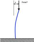 This equation is also used to obtain values for lateral deflections of the beam, by integrating twice to get y in terms of moment M and distance along beam, x. As mentioned in the last article however, the solution for buckling obtained from this equation has a trigonometric form (i.e. involving Sin and Cosine functions). To obtain the buckling load, it is assumed that the buckled beam has a shape defined by the bending equation. It follows from this that the applied load F, due to its eccentricity, causes the moment M (i.e. F.y = M).
M = F.y is substituted into the bending equation, to give a second order differential equation in y, the solution of which is known to be trigonometric. The noteworthy part of this approach is that the buckled shape of the beam has been assumed beforehand. In the preceding article it was stated that, to carry out a modal frequency solution in FEA, the equation:
requires an assumption that the displacement vector {X} is simple harmonic:

The connection between Euler buckling and modal analysis can now be seen: the solution is trigonometric. For a modal analysis, the equations of motion have a time-based, trigonometric solution for {X}. For the Euler buckling problem, static equations are derived with an assumed trigonometric form for {X}, in terms of the spatial co-ordinates.
As for a modal analysis, there are multiple results from a buckling FE analysis, consisting of a number of buckling load factors and corresponding mode shapes. The lowest load factor is usually the only one of practical interest.
The simple linear buckling method described does not take into account any initial defects in the structure and so the results are rarely conservative: that is to say that this type of solution usually over-estimates the buckling load. In practice it may be necessary to carry out a non-linear displacement analysis, using either an explicit or implicit solution.
Time based analyses – Implicit and Explict Solvers
Many types of non-linear analysis, like modelling slow contact between separate parts, for example, will require an analysis where the load is applied in several steps. In reality, the time over which the load is applied is not relevant but, for convenience, the steps in the analysis are applied over a specified time period of say one or ten seconds (sometimes called pseudo-time). This can be contrasted with a transient vibration analysis for example, where the real time over which the load is applied (and hence its frequency components) is fundamental to the analysis.
Both of the above problems can be carried out by finite element solution codes that use an ‘implicit’ method. The majority of mainstream and ‘traditional’ FE codes use this method. Other codes, many of which have been developed to deal with high-velocity impact problems like crashworthiness analyses, for example, use ‘explicit’ methods. The terms ‘explicit’ and ‘implicit’ refer to the numerical iteration technique used by which, having found a solution at one-time step, the solution at the next is obtained.
In an implicit solution, global equilibrium is achieved by iteration, after which local element variables are evaluated. Providing equilibrium can be achieved, there is no limit to the size of the time step that can be used. Hence, implicit schemes are termed ‘unconditionally stable’. Achieving global equilibrium at each time step involves matrix factorisation, however, which is computationally intensive. Analyses that are well-suited to implicit solution techniques are static, low-speed dynamic, or steady-state transport analyses.
By contrast, explicit solution techniques evaluate local variables directly, without the need for global equilibrium calculations. This benefit is offset by the need for calculations to be performed at small increments in order to maintain numerical stability. Significant errors develop if the time step size is too large. Hence, explicit schemes are termed ‘conditionally stable.’ Problems well suited to explicit solution are simultaneous large displacement and contact problems, rapidly changing or discontinuous loading, and rigid body motion.
Go to the next Knowledge Base article: Assessing Errors in Analysis Models or go back to Knowledge Base article series list