Nominal and Non-linear Stresses

Part 1

International standards and codes of practice enable engineering design to draw on the best available data from a history of testing and service experience. The last Knowledge Base article discussed using FEA in conjunction with two standards for the fatigue design of steel and aluminium structures (BS 7608:1993 and BS 8118- 1:1991). However, such codes often have inadequate guidelines on how to determine the required loads or stresses from FEA. The codes generally instruct on how to determine a nominal or net section stress which is intended to ignore the effect of local stress concentrations (notches) such as fillet radii, holes, changes in section or welds, the peak stresses arising from these being accounted for in the allowable stress values given in the two standards above. The nominal stress is intended to be a relatively easily calculated direct or bending stress, derived from the applied loads. Although offering many advantages, one difficulty when using FEA is identifying a point or region in a continually varying predicted stress field where the stresses can be regarded as representing the nominal values required by the code.

Sharing some features of the weld fatigue codes, widely used standards for the qualification of pressure vessels are the ASME Pressure Vessel code and BS PD 5500. In these codes, the two classes of stress termed primary and secondary share similarities with the nominal or net section stress and the not calculated but implied peak stresses around welds in the weld fatigue codes. However, in the pressure vessel codes, this distinction between primary and secondary stress is also derived from a consideration of proven failure modes - if the secondary stresses around a notch feature in a vessel exceeds the material yield strength the reduced stiffness of this region as a result of its yielding could start to fail if it were not for the support from the surrounding material (assuming sufficient ductility). Conversely, primary stresses that have exceeded yield would imply the whole cross-section of the vessel was yielding and failure is likely.

Consequently secondary stress, unlike primary, can be allowed to exceed yield without risk of failure, according to the pressure vessel codes. The fact that the code specifies a maximum allowable secondary stress at precisely twice yield is based on a more sophisticated argument, concerning failure due to cyclic loading, known as shakedown (stable stress-strain cycles with no failure) or ratchetting (increasing stresses and strains, leading to failure).

In order to understand shakedown and ratcheting, as well as other analysis applications such as limit analysis and impact damage assessments (to be discussed in future articles), it is necessary to examine some ideas behind mathematical material models used for structural metals.

Ordinary linear elastic FEA requires a single stiffness value, the Young’s Modulus (E) of the material. This is the gradient of the stress-strain curve and implies that the strain (or deflection) at any point increases proportionately to the stress (or load). This material proportionality prevails as long as the yield point (more formally, the limit of proportionality) is not reached.

A linear elastic FEA would substantially over-predict stresses that have exceeded the yield stress, but if the region of yielding around a notch is small, the approximate size of the region and the sub-yield stresses predicted by the linear FEA, away from the yielded region, can still be accurate.

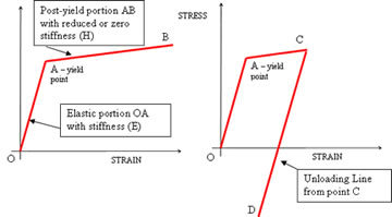
To have some chance of correctly predicting structural behaviour in parts of the structure where the yield point has been reached, the FEA material model needs to represent not only the shape of the stress-strain curve beyond the yield point but also the unloading behaviour of the material. The former is achieved by extending the linear elastic model, specifying the stiffness value (E), valid up to the yield point, and a further value or values, representing the post-yield stiffness (sometimes tangent stiffness, H). Even though the two gradient curve shown in the first diagram would not be a very good visible fit to the actual post-yield stress-strain curve of a typical engineering steel for example, such a bilinear model is often sufficient for reasonable conservative estimates of postyield behaviour in many applications. (More information on material models can be obtained in a recently published NAFEMS guide – ‘An Introduction to the Use of Material Models in FE .’)

The unloading behaviour, for loads up to the yield point A, is elastic, i.e. the stress and strain relationship at any point in the structure will be defined by points along the line OA for all loading and unloading. If the yield point is exceeded, however, the stresses on unloading will follow a line parallel to OA. The second diagram shows loading along OAC and unloading to a negative residual stress and positive residual strain, at D. At points within and around the yielded region, the unloading is not usually returned to either a zero stress or zero strain state, due to the constraint effects of the surrounding material. Hence there will be a spatial distribution of residual stresses and strains through the structure, after the external load is completely removed.

Part 2: Cyclic Plasticity

This article extends the introduction to modelling plastic or post-yield material behaviour introduced in the previous article. Plastic stresses first occur at stress concentrations or notches. These are termed secondary stresses in the context of the pressure vessel codes. Important concepts in cyclic or fatigue loading of components where the yield stress is exceeded will be explained.

High cycle fatigue refers to problems when the number of cycles to failure (or life) typically exceeds 105. In order to sustain this number of stress cycles, peak stresses are substantially lower than the yield strength of the material. This is therefore a simpler problem in principle than dealing with plastic cyclic stresses. The well known stress-life (or S-N) curve is pivotal in determining high cycle fatigue lives. In Figure 1, repeated from the previous article, this corresponds to stress cycles along the line OA. When stresses are high enough to cause plasticity to change during the load history, no equivalent of the S-N curve is available. Referring to Figure 1 again, if the yield point is exceeded, the stresses on unloading will follow a line parallel to OA. The diagram shows a particular case of loading to point C and the corresponding unloading to a negative residual stress and positive residual strain, at D.

At points within and around a substantial yielded region, the unloading (or the position of D) is not usually returned to either a zero stress or zero strain state, due to the constraint effects of the surrounding material. However, if the region of yield is small, which is consistent with the concept of secondary stress, the surrounding structure forces the region to a state of zero strain, indicated by point E in the diagram.

Considering the case of full unloading to zero strain at E, subsequent repeated application of the load will cause the straight line stress strain curve EC to be followed. So, after an initial over stress at this point in the component, subsequent cyclic stress cycles are elastic and the fatigue life should be close to that predicted by the high cycle S-N fatigue curve. However, at some peak stress higher than C, plasticity will occur during both unloading and subsequent reloading. In pressure vessel applications, it is often required to determine whether such plastic cycling is stable. Repeated applications of a cyclic load will result either in the plastic region expanding through the component section on each load cycle until failure occurs (perhaps after a very few cycles), or until the size of the plastic region stabilises with a higher or much higher number of cycles to failure. These are respectively termed ratchetting and shakedown.

In Figure 2, the line HIJ represents the stress-strain excursion from peak load to zero strain. This new shaped unloading line is due to the peak stress H, which is greater than C in Figure 1. The first portion of the unloading stress-strain curve HI is, like curve CE, parallel to the elastic line OA. Line HI is the same length as A` A, where A` represents the negative yield point. As the small region of plasticity is driven to zero strain by the surrounding material, what might be called the unloading elastic limit is reached at point I. The remainder of the trajectory to zero strain is therefore reached along the plastic line IJ, which is parallel to AH.

Subsequent reapplication of loading will follow the stress-strain curve towards K. The important difference between the two diagrams is that reloading in Figure 2 defines a new stress-strain path JK rather than following the previous path. This effect is called plastic cycling or hysteresis – the important phenomenon here is that plastic work is occurring to the material not only for the first cycle but also in subsequent cycles. Detailed numerical analysis is the only option to establish whether the plastic cycling is stable or propagates throughout the section, leading to failure or gross deformation.

The geometry of these simple stress-strain curves can be investigated to show that the limiting peak strain at which the transition to plastic cycling occurs (the transition between the first and second diagrams) is twice the yield strain. This is a useful conservative working figure used in the pressure vessel codes for guarding against ratchetting.