Modelling Wire Arc Additive Manufacturing

Authors: Yongle Sun | Cranfield University; Sjoerd Van-Der-Veen | Airbus; Anas Yaghi | TWI; Enrique Escobar de Obaldia | Ansys; Yupiter HP Manurung | SMRI; Marton Groza | NAFEMS

Reviewed and endorsed by the NAFEMS Metallic Additive Manufacturing Focus Team

S​upplementary Data

The NAFEMS Metallic Additive Manufacturing Focus Team, part of the Manufacturing Process Simulation Working Group, published their first example problem, ‘Predicting Buckling due to Thermal Distortion’ [1], in the 2024 October issue of Benchmark Magazine [2]. In this second example, the focus is on the resulting distortion and residual stresses from the Wire Arc Additive Manufacturing (WAAM) process. The problem statement has been extracted from the research of J. Ding et al. [3][4].

WAAM is a Directed Energy Deposition (DED) process that builds metal components by depositing weld beads layer by layer using an electric arc as a heat source and a filler wire as feedstock. WAAM enables high deposition rates and the fabrication of large structures at low cost, which is especially attractive for steel components in construction and shipbuilding, and high-value high-performance metal components in aerospace. The process involves intense localised heating and rapid cooling cycles, leading to significant residual stresses and deformations (distortion) in the built parts [5]. As the material is deposited in layers using high-intensity heat sources like arc welding, different regions of the workpiece experience varying temperatures. This leads to differential thermal expansion and contraction, usually accompanied by plastic deformation, which in turn creates internal stresses and can cause the workpiece to warp or distort. Although clamping or other restraints can suppress distortion during deposition, distortion may still occur after the restraints are removed due to the redistribution of residual stresses.

To address the challenge of residual stresses and distortions in WAAM, several strategies are employed. Techniques such as pre-bending, thermal and mechanical tensioning, and optimised deposition sequences help control stress buildup by manipulating the workpiece and deposition parameters during the manufacturing process. The approaches mentioned can significantly benefit from, or even essentially require, reliable Finite Element (FE) modelling techniques predicting distortions and stresses.

Modelling the WAAM process and the resulting residual stresses is challenging due to the complex thermal-mechanical phenomena involved. Nonetheless, in the past ten years, significant progress has been made in numerical simulations of WAAM, enabling researchers to predict residual stress distributions and distortion for various materials and process conditions. Approaches include detailed thermo-mechanical FE analysis [6] (Goldak double-ellipsoid heat source calibrated to thermocouple data; austenite-martensite phase transformation modelling with transformation-induced plasticity), the use of the inherent strain method [7] (calibrated from a small-scale simulation, and then applied layer-by-layer in a static mechanical analysis), and data-driven models [5] (numerous single-layer WAAM FE simulations are conducted, then Artificial Neural Network and Random Forest models are applied to predict residual stresses).

Modelling residual stress and distortion in WAAM is inherently a Multiphysics and Multiscale problem that stretches current simulation capabilities. Thermal gradients drive the need for fine resolution; phase transformations require coupling metallurgy with mechanics; multi-layer deposition demands long-sequence simulations or clever simplifications; material behaviour changes with temperature and microstructure, adding uncertainty; and the computational load is high. These difficulties mean that no single model can yet universally and efficiently predict WAAM residual stresses for all cases, and consequently, simulation engineers must balance accuracy and practicality.

The current set of well-documented measurement results aims to provide an example problem and the associated validation data for the comparison of different modelling techniques.

Experimental Setup

Sample walls were fabricated with 1, 2, 3, 4 and 20 layers using WAAM with mild steel on S355JR-AR grade rolled structural steel plates. The structure was cooled between depositing the layers using a water-cooled aluminium backing plate, with temperatures monitored using thermocouples to ensure optimal cooling and deposition conditions. The base plate dimension of the samples was 500 mm long, 60 mm wide and 12 mm thick. The multi-layer wall shaped samples were deposited along the centreline of the base plate with an approximate width of 5 mm and an average height of 2 mm for each layer. The welding process parameters utilised in these experiments were obtained from a preliminary process model study to achieve a specified target wall.

Thermocouples TP1, TP2 and TP3 were directly welded to the base plate surfaces, and TP4 was welded in a drilled hole which was four millimetres deep relative to the back surface.

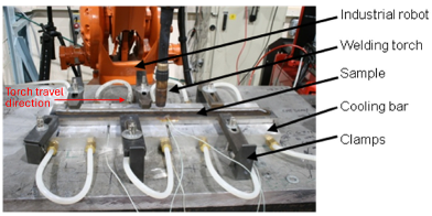
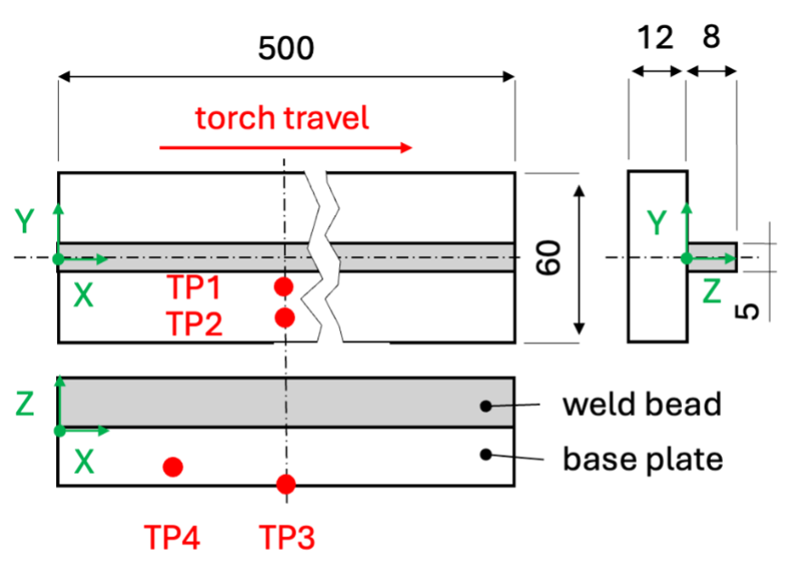
Figure 1 displays the experimental setup. Figure 2 shows the geometry of the test specimens for the 4-layer samples, the positions of the thermocouples, and the coordinate system used to define their positions. Table 1 summarises the clamping positions and Table 2 lists the positions of the thermocouples in the coordinate system used.

Figure 1: Experimental setup for the WAAM process and temperature measurement [1].

Figure 2: Geometry of the 4-layer test specimen, and positions of the thermocouples in a selected Cartesian coordinate system (unit: mm).

Table 1. Clamping positions estimated from experimental setup in Figure 1 (units in mm).

Note: In the deposition experiments, the clamping positions were not precisely controlled, and slight deviation was anticipated between different samples.

Table 2. Positions of the thermocouples (units in mm).

Table 3. Test specimens with different numbers of layers but same WAAM process parameters.

Process Parameters

The WAAM process adopted a Cold Metal Transfer (CMT) welding power source (a variant of Gas Metal Arc Welding (GMAW) adapted for controlled dip transfer mode), and the system was configured with a power input of 2495.4 W (averaged over the electric arc voltage and current cycles). The welding filler wire used in this study was 0.8 mm in diameter, and the wire feed speed was set at 10 m/min, complementing a torch travel speed of 8.33 mm/s in a single direction (Figure 1). The net heat input of the welding process was 269.6 J/mm, assuming an energy transfer efficiency of 0.9. Water-cooled aluminium backing bars were utilised to cool the sample more rapidly. Six clamps were utilised to fix the base plate to the cooling bars. To manage heat buildup and ensure consistent thermal condition between layers, the initial temperature before first layer deposition was about 24 °C and the interlayer dwell time remained constant for 400 seconds in each layer with the interlayer temperature kept in the range of 25-40 °C, as recorded by the thermocouples.

Material Properties

Table 4 and Table 5 summarise the chemical compositions of the S355JR-AR substrate plate and the deposition wire, respectively. Table 6 contains the thermal conductivity and the specific heat in function of the temperature for both the base plate and filler metal and Table 7 contains the mechanical properties. Above the melting temperature, the thermal conductivity is artificially increased to a high value to approximately account for the enhanced heat transfer caused by liquid-metal convection in the melt pool. The material used in the WAAM process exhibits a latent heat of 270 kJ/kg between temperatures of 1450°C and 1500°C. Material properties related to solid state phase transformation (SSPT) are not provided here. It is widely recognised that SSPT hardly affects the residual stress and distortion in mild steel, which experiences SSPT at high temperature, while SSPT would need to be considered in modelling for other materials (e.g. steels subject to martensite transformation at low temperature).

Through a thermal model calibration against the thermocouple data, the values of radiation emissivity and surface convection coefficient leading to the best prediction were identified. The radiation emissivity is 0.2 and the convection coefficient for the substrate and wall is 5.7 W/(m²K). An equivalent convection coefficient of 300 W/(m²K) was also determined for the bottom surface of the substrate, which represents the heat dissipation by the water-cooling back bars underneath the substrate.

Table 4. Chemical composition (in wt%) of the substrate plate (rolled structural steel grade S355JR-AR).

Table 5. Chemical composition (in wt%) of the deposition wire (mild steel).

Table 6. Thermal conductivity and specific heat in dependence of the temperature (Density (kg/m³) = 7860) [8].

Table 7. Temperature dependent mechanical properties for the substrate and the filler metal (ε_p: plastic strain) [8].

Experimental Results

Temperatures

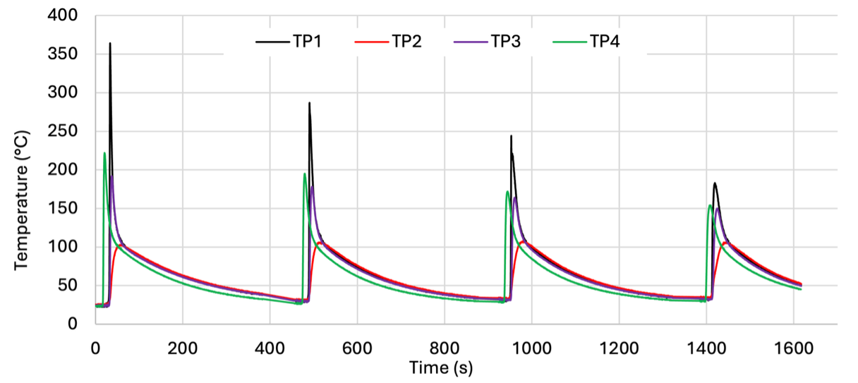
When conducting a sequentially coupled thermal–mechanical simulation, temperature results can be useful for conducting a verification step or, alternatively, for calibrating the transient thermal analysis. Temperature measurements were taken using four K-type thermocouples, which were welded at specified positions on the base plate (Figure 1 and Figure 2). The results are displayed in Figure 3 and are provided as supplementary downloadable data [9].

Figure 3: Temperature histories measured using four thermocouples installed at different locations in the base plate. [4].

Metallurgical Observations

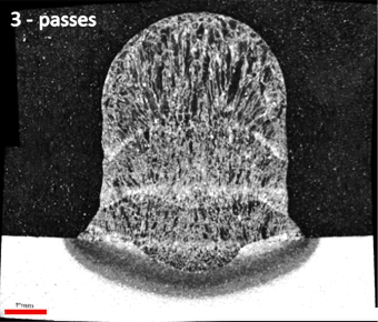
The fusion boundary and Heat Affected Zone (HAZ) boundary can be observed on the macrographs displayed in Figure 4 and Figure 5. The fusion boundary and HAZ boundary correspond to the melting temperature and austenisation temperature, respectively, and therefore they can be useful for checking the temperature prediction of the thermal analysis. In addition, the actual bead profile can be extracted from the macrograph for realistic geometry definition in a WAAM model.

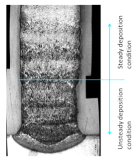
The blue line in Figure 5 highlights the slightly different resulting layer geometry and microstructure in the first few layers, due to the effect of the substrate, which can quickly dissipate heat with the aid of the back cooling bars. In these initial layers, the deposited beads are noticeably narrower, reflecting the stronger heat sink effect of the substrate; in some numerical models, this is explicitly taken into account by prescribing different bead geometries or process conditions for the first few layers. After deposition of more than 5 layers, the substrate effect was reduced and the WAAM deposition reached a steady condition, with more uniform bead width and microstructure along the build. In practice, one way to compensate for the initially narrower beads is to manually increase the power to obtain a wider melt pool in the early layers; however, this adjustment was not applied in the samples presented here.

Figure 4: A macrograph of the three-layer deposited wall (scale bar: 1 mm) and the neutron diffraction residual stress measurement position (red dash line) in the base plate (S3 sample) [4].

Figure 5: A macrograph of the 20-layer deposited wall (scale bar: 1 mm), S5 sample [4].

Elastic Strain Measurement Using the Neutron Diffraction Method

The lattice strain (i.e. elastic strain) induced by the WAAM process was measured using a neutron diffraction strain scanner (ENGIN-X at ISIS, Oxford, UK). Elastic strain was measured in longitudinal, transverse, and build directions after the clamps were removed at room temperature. The gauge volumes were 2×2×2 mm³ for longitudinal measurements and 20×2×2 mm³ for transverse and build measurements. The choice of a larger gauge size in the longitudinal direction, 20 mm, was beneficial for reducing measurement time, which did not impair the accuracy as the measurement was performed in the mid-length region, where the stresses were approximately uniformly distributed in the longitudinal direction. The strain measurements were performed along a transverse line 2 mm below the top surface of the base plate for the S1, S2 and S3 samples, while the measurement path was along the through-height direction in the mid-width plane for the S5 sample.

Residual Stress in the Substrate

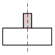
Hooke’s law was employed to derive the residual stress from the neutron diffraction strain measurements using ambient temperature properties along the red dashed line displayed in Figure 6 in mid-length plane. The longitudinal (X), transverse (Y) and build direction (Z) components of the residual stress are provided as supplementary downloadable data [9]. The stress measurement error was estimated based on the uncertainty associated with neutron diffraction peak fitting, which influences the determined lattice spacing.

Figure 6: Path of the residual stress measurement in the substrate (S1, S2, S3 samples).

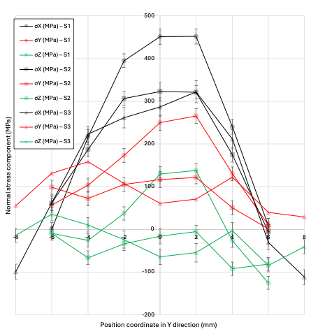
Figure 7 shows the measured residual stress components in substrate (S1 sample) with 1 confidence interval (half-width of a symmetric (two-sided) confidence interval centred on the best estimate).

Figure 7: Measured residual stress components in substrate (S1, S2 and S3 samples) with 1 confidence interval.

Residual Stress in the Wall

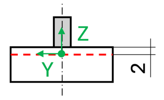
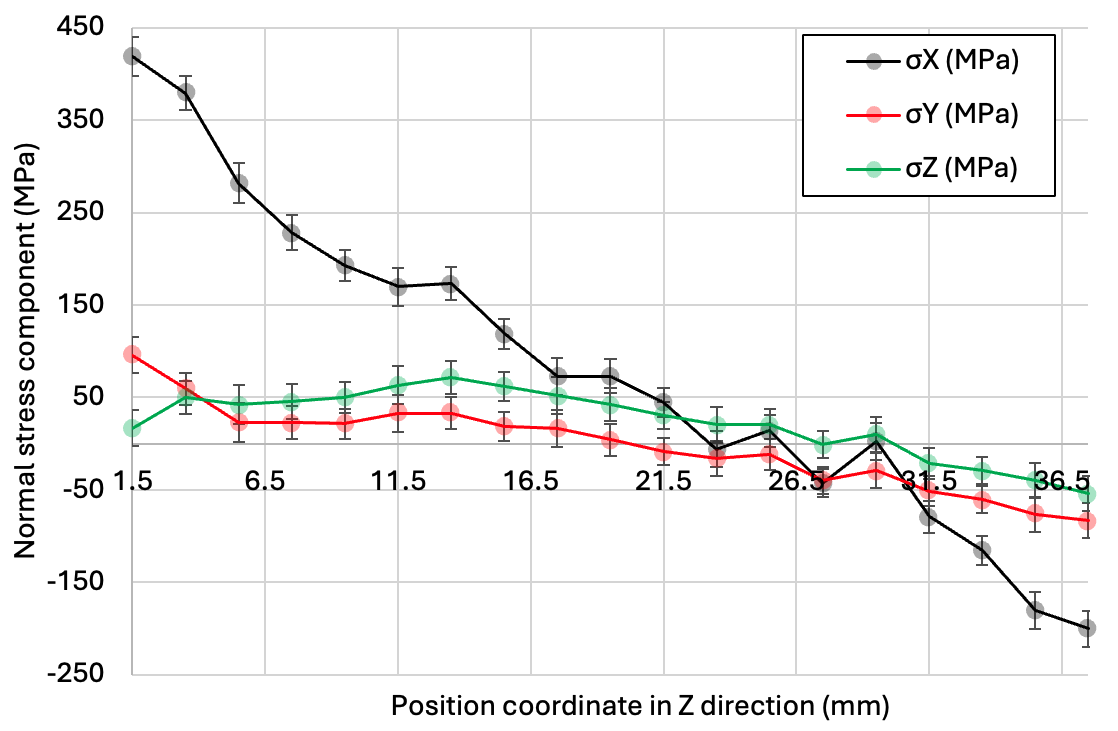
Residual stress was measured along the red dashed line displayed in Figure 8 in mid-length plane using the neutron diffraction method (measurement was conducted after removal of clamps at room temperature). The three normal stress components are provided as supplementary downloadable data [9]. The stress measurement error was estimated based on the uncertainty associated with neutron diffraction peak fitting, which influences the determined lattice spacing. Figure 9 displays the measured residual stress components in wall (S5 sample) with 1 confidence interval (half-width of a symmetric (two-sided) confidence interval centred on the best estimate).

Figure 8: Path of the residual stress measurement in the 20-layer wall (S5 sample).

Figure 9: Measured residual stress components in wall (S5 sample) with 1 confidence interval.

Distortion

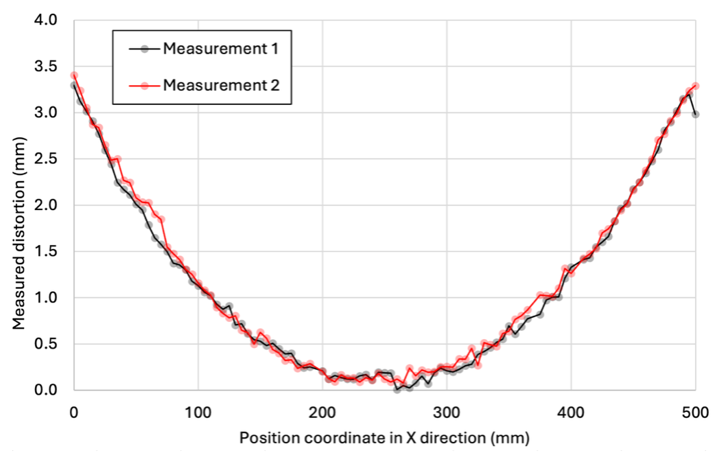
Distortion was measured using a Romer Omega Arm equipped with an R-Scan 3D laser scanning system. This setup allowed for detailed analysis of the distortion patterns and their magnitudes. The distortion measurement was conducted along the two long edges on the substrate bottom after removal of the clamps. The measured distortions are provided as supplementary downloadable data [9].

Figure 10: Measured distortion in 4-layer wall (S4 sample).

Modelling Guidance

To enable a meaningful comparison between different numerical approaches and to make best use of the experimental data, a common set of modelling assumptions is recommended. Within this common framework, participants are encouraged to explore different process modelling strategies and numerical implementations. The following guidelines summarise which aspects should be aligned across models, and which may differ.

All simulations intended for comparison against this example problem are expected to consider the following:

• Aim to predict both residual stress and distortion. The primary quantities of interest are the residual stress fields in the substrate and wall, and the distortion of the substrate after unclamping.
• Use the same material properties as provided. Temperature-dependent thermal and mechanical properties for the substrate and filler metal should be taken from Table 6 and Table 7. The latent heat associated with phase change may be neglected in the thermal analysis, provided that the resulting temperature histories remain in good agreement with the thermocouple measurements and metallurgical observations of isotherms.
• Include both clamping and unclamping. The mechanical analysis should explicitly represent the clamping conditions during deposition and the subsequent unclamping step, as these have a significant influence on the final residual stress and distortion states.
• Respect the as-provided wall and substrate cross-section. The width and height of the wall and substrate should follow the experimental geometry (Figure 2 and accompanying descriptions). Use the as-provided wall and substrate length for unclamping simulations. With the above implementation, the stress and distortion predictions are directly comparable to the measurements.
• For simulations that include unclamping and predict the final residual stress and distortion, the full specimen length (500 mm substrate) should be modelled. A reduced length may be used only for simulations targeting the residual stress state under clamped conditions, where end effects are not of interest.

Within the these constraints, different modelling strategies may be adopted to explore the trade-off between accuracy, robustness, and computational cost. The following aspects are allowed – and expected – to vary:

• Process modelling approach. Different representations of the thermo-mechanical behaviour may be employed, such as fully coupled thermo-elastic-plastic analyses, inherent strain methods, thermal shrinkage approaches, or data-driven / machine-learning-based models.
• Heat source model. Various weld heat source formulations may be used (e.g. double-ellipsoidal, single-ellipsoidal, circular, or other equivalent models). In all cases, the resulting temperature field should be calibrated and/or verified against the measured thermocouple histories and, where appropriate, metallurgical indicators for isotherms (fusion and HAZ boundaries).
• Layer activation strategy. Different techniques for adding material can be applied, including element birth and death, quiet elements, element-by-element activation, whole-layer activation, or lumped-layer approaches. The chosen strategy should be documented together with any mesh-related simplifications.
• Boundary conditions and constraints. Engineers may refine or recalibrate the thermal boundary conditions (e.g. convection coefficients, emissivity values, representation of the water-cooled backing bars) and the mechanical constraints (e.g. rigid versus compliant clamps, hard contact formulations, node fixities, use of symmetry conditions), provided these choices are consistent with the experimental setup.
• Modelled part size and symmetry. While full-length models are required for simulations including unclamping, reduced models (e.g. half models, shorter sections, or symmetry-reduced domains) may be used for parametric studies or for predicting residual stresses in the clamped condition, as long as end effects and boundary influences are appropriately considered. The bead section geometry could be extracted from the macrographs or simplified (e.g., a rectangle) using the measured average bead dimensions.

References

• [1] ‘Additive Manufacturing Simulation Example Problems’, Metallic Additive Manufacturing Focus Team, NAFEMS website. Available: nafems.org/community/working-groups/manufacturing-process-simulation/metallic-additive-manufacturing-focus-team/challenge-problems/ (accessed Nov. 30, 2025).
• [2] S. Van Der Veen, A. Yaghi, D. Afazov, T. London, Y. Sun, G. Vastola, M. Megahed, and M. Groza, ‘Predicting Buckling due to Thermal Distortion’, BENCHMARK, 1 Oct. 2024. Available: nafems.org/publications/resource_center/bm_oct_24_6/ (accessed Nov. 30, 2025)
• [3] J. Ding, P. Colegrove, J. Mehnen, S. Ganguly, P. M. Sequeira Almeida, F. Wang, and S. Williams, ‘Thermo-mechanical analysis of Wire and Arc Additive Layer Manufacturing process on large multi-layer parts’, Computational Materials Science, vol. 50, no. 12, pp. 3315-3322, 2011. [Online]. Available: doi.org/10.1016/j.commatsci.2011.06.023
• [4] J. Ding, ‘Thermo-mechanical analysis of wire and arc additive manufacturing process’, PhD Thesis, Cranfield University, 2012, [Online]. Available: dspace.lib.cranfield.ac.uk/handle/1826/7897
• [5] Q. Wu, T. Mukherjee, A. De, and T. DebRoy, ‘Residual stresses in wire-arc additive manufacturing – Hierarchy of influential variables’, Additive Manufacturing, vol. 35, 2020.
• [6] X. Jimenez, W. Dong, S. Paul, M. A. Klecka, and A. C. To, ‘Residual Stress Modeling with Phase Transformation for Wire Arc Additive Manufacturing of B91 Steel’, JOM, vol. 72, no. 12, pp. 4424–4433, 2020. [Online]. Available: osti.gov/servlets/purl/1842649
• [7] C. Behrens, S. Neubert, M. Siewert, M.S. Mohebbi, and V. Ploshikhin, (2023). ‘Integration of annealing into the inherent strain simulation of wire arc additive manufacturing’, Additive Manufacturing Letters, 4, 100115.
• [8] P. Michaleris and A. DeBiccari, ‘Prediction of welding distortion’, Welding Journal-Including Welding Research Supplement, 76(4):172s, 1997.
• [9] Supplementary Data for the current article ‘Modelling Wire Arc Additive Manufacturing’.

Acknowledgement

The authors wish to take this opportunity to thank the NAFEMS Metallic Additive Manufacturing Focus Team members for their help and support in the preparation of this article.

Within the NAFEMS Community, the Metallic Additive Manufacturing Focus Team, part of the Manufacturing Process Simulation Working Group, is dedicated to fostering collaboration between industry and academic experts and developing technical resources in this field.